|
|
Basic Matlab
Graphing
Steve
Seow
Brown
University February
2003 Originally prepared for
PY107 Psychological
Theory with Professor Russell M.
Church Spring 2003 Brown University This document provide
a step-by-step tutorial on creating a simple graph in Matlab. All codes
and data appear in courier font. The color
coding is somewhat consistent to what you would see in Matlab if you were
to type the line in the command window or in the
debugger/editor. 1. Getting acquainted
with plot
function There is more than one way to create simple graphs in Matlab but for starters, we’ll just deal with the basic stuff. If you simply type plot in the command window and hit enter, you will see... >>
plot ???
Error using ==> plot Not
enough input arguments. >>
This is because you
need to tell Matlab what to plot. If you type
>>
plot(x) ???
Undefined function or variable 'x'. >>
This failed again
because x has not been defined.
This is Lesson No. 1: you need have data in some form to use the
plot function. Let’s
define x by
typing
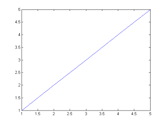
>> x = [1 2 3 4 5] x
= 1 2 3 4
5 >>
Now try plotting x
again by typing plot(x)on the command window.
A new window should appear with a graph that looks something like this:
2. Plotting two
vectors There is a few
problems in the graph above. For a start, we can’t really tell what is
being plotted against what. Typically we want to plot one vector against
another. As such, we’ll create a second vector and we’ll call it
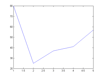
y. >> y = [80
25 37 41 57 23] y
= 80 25 37 41 57 23 >>
We’ll plot vector y as
a function of x
by using
the simple command plot(x,y). Hit the enter key and you’ll get the following message:
>>
plot(x,y) ???
Error using ==> plot Vectors
must be the same lengths. >>
Lesson No. 2: The
lengths of the vectors you use in a plot command must be
equal. Type size(x) and size(y) to display the
dimensions of the vectors. You will notice that y
is one
element longer than x.
Suppose
that the length problem is corrected in that both x and y have 5 elements. If
we retype the command plot(x,y)and hit enter. Nothing
happens. Why? Lesson No. 3: New
figures are plotted over and overwrites old ones. Click on the first
figure and you will notice that it has changed and it looks different from
the one above.
If you want to preserve the previous figure and create a new one in a another window, use the figure command before plotting the next graph. >>
figure >>
plot(x,y) >>
3. Markers and
Lines Needless to say, the
graph above needs a lot of work. Typically, we would like to see where the
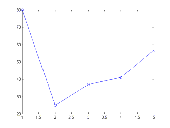
coordinates are. To put markers on the graph, we’ll modify the
plot(x,y)line into plot(x,y,'o-b')and this is what we
get:
The 'o-b'
argument
tells the program to plot the graph with open blue circles and blue lines.
The o
can be
substituted with a variety of shapes, such as * for a start,
d for a diamond,
. for a dot,
<, >, and ^ for triangles. The –
tells the program to use lines in between the markers. This can also be
substituted for a variety of line types, such as -- for dashed lines and .- for dashdot lines.
The b part tells the
program to use blue color for the lines and markers. A complete listing of
types of markers, lines, and colors can be found by typing help
plot at
the command window. 4. Axes Labels and
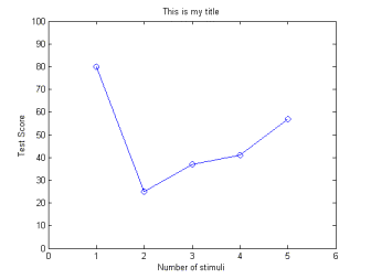
Title A proper graph should
have a title and correctly labeled axes. Labeling the x- and y-axis in
Matlab can be performed by running the appropriate commands. Suppose we
want to label the x axis as “Number of stimuli”, we would use the command
xlabel('Number of stimuli').Labeling the y axis is
similar in that you use ylabel instead. To entitle
the graph, we would use title('This is my title'). The following is an
example of a graph with labeled x- and y-axis and a
title:
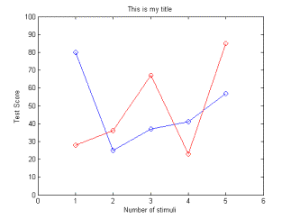
5. Axis
Scales It is possible to
modify the x- and y-axis in our example above so that both starts at 0 (if
necessary). To do this add the line axis([0
6 0 100])
, where the first two numbers refer to the minimum and maximum values on
the x-axis, followed by the minimum and maximum values of the y-axis. The
graph should now look like this:
6. Plotting another
vector into existing graph Sometimes it is
necessary to add another vector or series into an existing graph. To do
this, we need to use the hold
on
command. Suppose we want to graph both x and a new vector
called z into the graph, we
would insert a hold
on
command after plotting one vector:
>> plot(x,y,'o-b') >> hold on
>> plot(x,z,'o-r')
This will produce a graph that looks like
this:
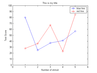
7.
Legend It is always good
practice to provide a legend if more than one vector is being plotted. To
create a legend, we’ll add the command legend('blue line','red
line'). The program will
assign the name blue
line to
whichever vector was plotted first, and red
line to
the second. By default, the legend will be added to the top right corner.
This position can be change by adding an argument at the end of the names,
such as legend('blue line','red
line', 2)to place the legend on
the top left corner. Try using arguments 0 through 5 to see what
happens.
8.
Summary We summarize all the commands necessary to get to the figure above. This is typically constructed in the Debugger/Editor and executed as an m-file. If these lines are copy and pasted into your command window, it should produce the same figure as the one above. x
= [1 2 3 4 5 ] y
= [80 25 37 41 57] z
= [28 36 67 23 85] figure plot(x,y,'o-b') hold
on plot(x,z,'o-r') axis([0
6 0 100]) xlabel('Number of stimuli') ylabel('Test Score') title('This is my title') legend('blue line','red line') |
|